Real-time Object Detection Using Faster R-CNNs
April 20, 2018Introduction
In this post we will talk about the object detection system using Faster R-CNN proposed by Ren et. al. in 2015. Faster R-CNNs are made up of two modules. The first one is a fully convolutional network called the Region Proposal Network (RPN) and the second module is the Fast R-CNN detector that uses the proposed regions for classification. The entire system is one single combined system for object detection. The RPN module tells the R-CNN where to look. The following figure shows the Faster R-CNN.
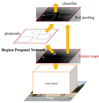
Faster R-CNN is a single network consisting of 2 modules. The RPN modules serves as the 'attention' for the unified network. (Source:https://arxiv.org/abs/1506.01497)
Faster R-CNN
Now we talk about the different components of the Faster R-CNN in detail
Region Proposal Networks
An RPN takes as input an image and returns a set of rectangles, these are the object proposals and each of them has an objectness score. This is done using a fully convolutional network, which shares some convolutional layers with a Fast R-CNN object detection network. The regions are generated by using a small network over the convolutional feature map. This feature map is the output of the last shared convolutional layer. The small network takes as input a n x n region of the feature map, which is then mapped to a lower-dimension feature with 256 layers (filters), 256-d. These are input into two parallel fully connected layer, a box-regression layer (reg) and a box-classification layer (cls). Ren et.al take the value n = 3 for their paper. This mini-network consists of a $n \times n$ convolutional layer, followed by two siblings convolutional $1 \times 1$ layers, the reg, and cls respectively.
Anchors
For each sliding window, the networks make multiple simultaneous proposals, where is the number of proposals for each sliding window location is k. The reg layer gives 4k outputs containing the coordinates of the k boxes and the cls layer had 2k scores that estimate the probability of being an object or not object for each proposal. These k proposals are estimated from k reference boxes, which are called anchors. An anchor for a given sliding window, has a scale and aspect ratio associated with it, in their paper Ren et. al have used 3 scales and 3 aspect ratios, this yields 9 anchors at each sliding window location. For a convolutional feature map of size $w \times h$ the total number of anchors = $w \times h \times k$.
Transition-Invariant Anchors
This way of selecting anchors make them translation invariant. It basically means that if one translates an object in an image, the proposal should also translate and the same function would be able to predict the proposal in either location. The translation invariant reduces the model size as well. For example the MultiBox method [2] has a $(4 + 1) \times 800-dimenetional$ fully-connected output layer, whereas this method just has $(4 + 2) \times 9$-dimensional convolutional output layer in the case of $k=9$ anchors. Due to smaller datasets, there is also a lesser risk of overfitting on smaller datasets like the PASCAL VOC.
Multiscale Anchors as Regression References
Instead of resizing images for computing the features at each scale, it is faster to use a sliding window of multiple scales on the feature maps. Ren [1], uses the idea of pyramid of anchors, which is similar to the DPM[], where models with different aspect ratios are trained using different filter sizes, “pyramid of filters”. The method classifies objects and regresses bounding boxes based on the anchors of different sizes and aspect ratios, on feature maps and filters of a single scale. Similar to the Fast R-CNN detector[], Faster-RCNNs use the convolutional features computed on a single scale image, which is the key component for sharing features without any extra cost related to varying image scales.
The Loss Function
RPNs are trained using the anchors where each of them is assigned a binary label of being an object or not. A positive label is assigned to the anchor with the largest intersection-over-Union (IoU) overlap with the ground truth box, or an anchor with IoU greater than 0.7. Both these conditions are required to ensure there are positive anchors for all cases. Negative labels are assigned to a non-positive anchor whose IoU is less than 0.3 for all the ground-truth boxes. Anchors that remain unlabelled are not considered in the training process. Thus the objective function is minimized using the following loss function for an image:
Training
The RPNs are trained using back-propagation using stochastic gradient descent (SGD). Each mini-batch is derived from a single image that contains several positive and negative anchors. The mini-batches consist of positive anchors and negative anchors in the ratio of approx $1:1$, if there are less than 128 positive anchors for an image, they are padded with negative anchors.
The shared convolutional layer is initialized using weights from a model trained on ImageNet Classification. The new layers are initialized with random weights taken from a zero mean Gaussian distribution with standard deviation of 0.01. The leaning rate of 0.0001 is used for the first 60k mini-batches and 0.0001 for the next 20k mini-batches on the PASCAL VOC dataset. The momentum of 0.9 and weight decay of 0.0005 has been used.
Sharing Feature training for RPN and Fast R-CNN
Now we consider the object-detection CNN which will be utilizing the regions proposed by the RPNs. For this, we use Fast R-CNN [1]. Next we talk about algorithm used to train a combined RPN and Fast R-CNN having shared convolutional layers, as shown in the Introduction.
4-step alternating training has been used in the Faster R-CNN approach.
- The RPN is trained using the several anchors as discussed earlier. This network is initialized with an ImageNet pre-trained model and then trained end-to-end for region proposal task.
- A separate detection network is now trained by Fast R-CNN, using the proposals generated by the RPN in step 1. This network is also initialized by the ImageNet pre-trained model.
- Next, the detector network is used to initialize the RPN training, the weights on the share convolutional layers are fixed and only the layer unique to the RPN are altered. Now the layers share some convolutional layers.
- Keeping the shared convolutional layers fixed for the layers unique to the Fast R-CNN are trained.
These step may be repeated for more training, but it leads to negligible improvements.
Implementation Details
Both the RPN and the object detection network on images with single scale. Images are rescaled such that their shorted side, $s = 600$ pixels [2]. For anchors, boxes with are $128^2$, $256^2$ and $512^2$ is used with the aspect ratios, 1:1, 1:2 and 2:1. Both ZF net and VGG nets were used for initializing weights for the RPN. There are anchor boxes which cross the boundaries of the image, during training, such anchors have been ignored. For a typical $1000 \times 600$ image there are approx. 20000 anchors. Ignoring the cross-boundary anchors, this falls to around 6000 anchors per image. if not ignored, the cross-boundary anchors introduce large errors in the objective and the training does not converge. During testing the same RPNs are used, the cross-boundary proposals are clipped to the image boundary.
Some of the proposals are highly overlapping, to reduce this redundancy, a technique called non-maximum suppression (NMS) has been used. The cls score is used for the NMS and the IoU is set at 0.7. This means that if two proposal boxes have an IoU of 0.7, the one with the higher cls score is selected for training. Using NMS does not affect the detection accuracy and also reduces the number of proposals. Using NMS gives around 2000 proposals per image, which is used for training the Fast R-CNN. The top N-ranked regions are used for detection.
References
[1] R. Girshick, “Fast R-CNN,” in IEEE International Conference on Computer Vision (ICCV), 2015
[2] Ren, Shaoqing, et al. “Faster r-cnn: Towards real-time object detection with region proposal networks.” Advances in neural information processing systems. 2015.
Useful Links
Paper: https://arxiv.org/abs/1506.01497
Official repo: https://github.com/ShaoqingRen/faster_rcnn